Merging statistics and geospatial information, 2018 projects - Finland

Predict crop yields from a sequence of remotely sensed multispectral images; 2018 project; final report 31 December 2020

This article forms part of Eurostat’s statistical report on the Integration of statistical and geospatial information.

Full article

Problem

Farm surveys are very costly in terms of time and expense as is gathering expert estimates.

Objectives

The project aimed to predict crop yields from a sequence of remotely sensed multispectral images, where each image corresponds to a different day of the year within a growing season.

Method

Raster data from Copernicus Sentinel-2 Level 2A tiles were processed. Pixel values were extracted from images and these values were further compressed into histogram values. Scripts were run for the whole of Finland as the reference data of historical crop yields covered all arable land on the national territory. Time series were created for the growing season, from 1 May until 1 September: in practice data were available for 115 days from 10 May to 1 September. From the 13 spectral bands for Sentinel-2 images, 10 bands (2, 3, 4, 5, 6, 7, 8, 8A, 11 and 12) were used, each stored in a separate geoTIFF. For example, in 2018, there were 2.9TB of data from 42 930 images. The data were processed on a supercomputer. As well as the Sentinel-2 data, the main input is shapefiles showing field parcels. The required observation unit was the farm, made up of fields (polygons) or groups of fields (multi-polygon) if the same crop was grown on multiple fields of a single farm.

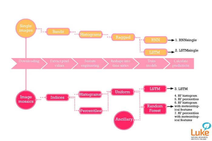
In practice, two approaches were taken, one using single images from Sentinel-2 data and the other using image mosaics. The first approach has the advantage of less pre-processing whereas the second reduced the data size for later processing.

For single images, pixel values were extracted from the images. These values were arranged polygon-wise into 32 bin normalised histograms. This resulted in a dataset of pixels organised into 115 time steps, 10 bands and 32 bins.
Index mosaics were created by assembling multiple overlapping images. An image mosaic is produced from the most optimal pixel values. The mosaics were computed on the 15th and on the last day of each month, giving two observations per month. For each mosaic, information for 30 days was compressed into one value, with the time series of mosaics overlapping by 15 days. The index mosaics used were the Normalised Difference Moisture Index (NDMI), the Normalised Difference Tillage Index (NDTI) and the Normalised Difference Vegetation Index (NDVI). The pixel values were arranged polygon-wise into 16 bin normalised histograms. This resulted in a dataset of pixels organised into 13 time steps, 3 indices and 16 bins. This was extended by adding meteorological information for seven dates for three indicators (precipitation, solar radiation and temperature).

Figure 1: Scheme for the model development

Three modelling approaches were tested: Vanilla Recursive Neural Network (RNN), Long-Short Term Memory Network (LSTM) and Random Forest (RF).

Results

From single satellite images Sentinel-2 data from 2016 to 2020 were processed. Two RNN models were produced from these data: RNNsingle and LSTMsingle. The image mosaics covered the years from 2018 to 2020. LSTMmosaic and RFmosaic models were produced from these data. The models were trained with data for 2016–2019 (single) or 2018–2019 (mosaic). The models were used to produce results for 2020 for four crop types: wheat (split between winter and spring), rye, barley (split between feed and malting) and oats. The modelled results were compiled in June, July and August as well as at the end of the growing season. These were compared with preliminary crop statistics available at the end of November each year from a survey of farmers as well as other forecasts produced by the Natural Resources Institute Finland (mid-July and end-August) as well as by the Joint Research Centre (mid-June, end-July and end-August).

The predictions by the models seemed accurate already in June. Neither the mosaic nor single models were superior in accuracy. RFmosaic, LSTMmosaic, and LSTMsingle seemed to be promising predictive models. The performance varies between crops. One of the main reasons for this is that the amount of training data greatly differed between crops. Adding meteorological features can improve the RFmosaic model, but only slightly.