Merging statistics and geospatial information, 2015 projects - Slovenia
This article forms part of Eurostat’s statistical report on Merging statistics and geospatial information: 2019 edition.
Final report 3 January 2018
Full article
Problem
A lack of geospatial data (for example, in the fields of income and health statistics) and the need to develop innovative approaches for treating confidentiality were two problematic issues identified by the Statistical Office of the Republic of Slovenia (SURS). They also identified that a great amount of computer coding would be required in order to develop a fully functioning system for the development of a GIS-based data viewer that allows geospatial statistical data to be published as free open data.
Objectives
The objectives of this project were to:
- establish two geospatial statistical databases, one on income and the other on health; for the latter develop estimation methods;
- examine and implement innovative approaches to statistical confidentiality;
- upgrade a web application called STAGE, in particular by making it accessible for small touchscreen devices.
Method
Geospatial statistical database on income statistics
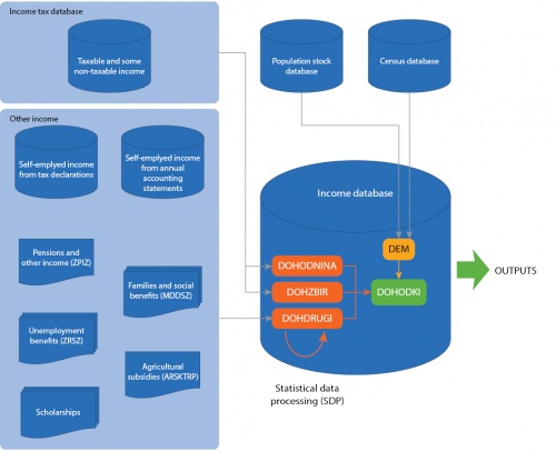
The population stock database and the register-based population and housing census (Census Database) were sources from the statistical office based on the central population register and the household register kept by the Ministry of the Interior (MNZ). It was decided to combine the income database with data from these two sources (for information on 31 December 2014 and/or 1 January 2015) with income data from 2014, available from a variety of sources, including:
- several tax sources from the Financial Administration of the Republic of Slovenia (FURS);
- unemployment benefits from the Employment Service of Slovenia (ZRSZ);
- parental and family receipts, scholarships from the Ministry of Labour, Family, Social Affairs and Equal Opportunities (MDDSZ);
- agricultural subsidies from the Agency for Agricultural Markets and Rural Development (ARSKTRP);
- pensions from the Pension and Disability Insurance Institute of Slovenia (ZPIZ).
An Oracle database was constructed, with procedures to extract, transform and load data from each of these sources.
The population stock database contained demographic data and geospatial data: 24 basic demographic variables (age, gender, residential status as of 31 December and majority of the year), derived variables (education, activity status, profession) and geospatial variables (cohesion region, statistical region, administrative unit, municipality, local community, settlement, spatial district, MID of the house number (XY coordinates)) for the entire population with registered permanent or temporary residence in Slovenia (and also some persons without permanent residence). These data were combined into one table — called DEM — along with the three household variables from the census database (updated every three or four years) and eight derived household variables (which enabled the calculation of poverty indicators).
The DOHODNINA table contained detailed income data from the income tax register. Net income was calculated for each type of income and sums of different kinds of income were also calculated. The DOHZBIR table contained 102 variables from the income tax register on final aggregate income, tax adjustments and reliefs, and income from abroad. The DOHDRUGI table contained detailed income data from all other sources: 195 variables. Data in these three tables were validated and corrected. All records containing income data were linked via personal identification numbers (SID) to the DEM table.
Geospatial statistical database on health statistics
A set of exclusion criteria were established to determine which health indicators would (not) be included in the database. In summary:
- data were not accessible at the municipality level (LAU 2);
- primary data were considered to be of poor quality;
- data were from a small sample survey;
- there were a small number of phenomena (for example, the low occurrence of specific diseases) in the population;
- data were collected only once, continuous/regular data collection was not expected;
- some similar indicators were duplicated, describing the same area/phenomena;
- some indicators were ambiguous, they did not reflect their purpose sufficiently;
- some indicators did not provide statistical support for decision-making, and would fail to invoke any action.
After discussions with stakeholders, 31 indicators were selected and grouped under four main chapters: risk factors, prevention, health status and mortality. The data sources used for these indicators were scattered among various institutions and among a variety of data environments.
Estimates for the whole set of heath indicators were calculated at the level of municipalities (LAU 2), administrative units (LAU 1), statistical regions (NUTS level 3), and the whole country. For most indicators three- or five-year moving averages were calculated to reduce the variability inherent in the occurrence of rare events, particularly in the smallest municipalities. Furthermore, for some indicators, information by age was standardised (based on the mid-2014 Slovenian age structure). As the data were age-standardised and presented as moving averages, further controls for statistical disclosure were regarded as unnecessary.
Thematic (choropleth) maps were produced for each of the indicators, showing data for 2012 municipalities. These maps were initially made available in a fixed (“printed”) format, with plans to disseminate them through the STAGE platform; it was planned to update the database on an annual basis.
Downscaling methods for sample surveys
While many health indicators came from exhaustive administrative data, there were a lack of indicators for measuring health behaviour, health determinants and the self-assessment of health and disability. Indicators for these issues generally came from sample surveys, with the drawback that their samples were often too small for an analysis of detailed territorial divisions, such as municipalities. It was considered difficult to simply increase sample sizes due to budget constraints, time constraints and the likely burden on respondents.
Several methodological approaches were available to overcome these challenges, for example, downscaling methods or small-area estimates. Initially, estimates were developed for the following indicators, selected from the 2014 European health interview survey:
- daily smokers of tobacco products;
- self-perceived health status (good and very good);
- binge drinking;
- people living with available help from their neighbours (if necessary).
Auxiliary variables from national healthcare administrative databases (NIJZ) and from the statistical office were used to improve estimates at the municipality level. Some were variables included in a new geospatial statistical database on health statistics. Others were from the statistical office and mainly concerned indicators at the municipality level that were generally associated with health outcomes and behaviours, including for the labour market, demographics, education, income, transport and environmental indicators.
Two modelling strategies were employed during the preparation of small-area estimates: generalised linear mixed models (using municipalities within administrative units as two random factors) and Bayesian modelling using R-INLA (using municipalities with their neighbours and Besag/BYM model), both within a binomial family. Given a choice of around 60 auxiliary variables, research was undertaken to identify which of these variables were associated with the dependent indicator. Several measures of a quality of fit were observed. At first, a dependent indicator (survey data) was modelled with each possible independent variable; then, a model was prepared containing expert-endorsed variables and a few other indicators that had a significant effect or a good fit in the univariate models. Serious deviances or unexpected values in some municipalities were identified and the model was adjusted. Both models (GLMM and Bayesian) were adopted and the value of their estimates were compared.
Statistical confidentiality
Income data are, in general, deemed to be sensitive, and there may be an increased risk of disclosure of income data when combined with geospatial information, particularly at more detailed levels. The statistical office has traditionally published data for NUTS regions, LAUs and also square grid cells with sizes ranging from 5 km² to 100 m². Traditionally, disclosure has been controlled through the use of cell suppression: if the frequency of observations in a specific cell was below a certain threshold, then the value for that cell was not shown.
The first step was to review the statistical disclosure control methods most commonly used with microdata and to participate in an international conference on privacy in statistical databases.
Two perturbative methods of statistical disclosure control were selected for testing which were designed specifically with geospatial data in mind. The first method was a record swapping procedure, intended to identify rare individuals at risk of disclosure according to a pre-specified set of variables. The disclosure risk was assessed at each geographical level. Those households where individuals were considered to be at risk of disclosure were then moved geographically by swapping their geographical variables (while keeping their other characteristics unchanged).
The second method chosen for further tests was a perturbative post-tabular method called the cell-key method. This method generated perturbations for small-valued cells in a consistent way, so that the cells consisting of the same individuals were always perturbed by the same value, even in different tabulations.
Preliminary tests were done on a set of demographic variables from the 2011 census. While swapping records only changed the total population count in a small number of grid cells the changes observed were sometimes large, for example if large institutional households were swapped. The cell-key method perturbed most of the original values, but the perturbations conformed to a pre-specified distribution and were mostly small, such that the total count was unchanged.
Further tests for the cell-key method were carried out for income data, looking at income quartiles for total gross income; the geospatial distribution of quartile sizes on a 5 km² grid was indistinguishable from the original distribution. The cell-key method, however, was originally intended for analysing frequency data and, it was considered that more generally, the statistical disclosure control method should be chosen to be congruent with the type of statistic it was meant to protect.
Income data characteristics were explored in more detail and a set of indicators from 2014 were chosen for mapping. The total gross annual income was chosen as the primary variable to be analysed. It was decided that the median (rather than the mean) should be reported as an indicator of central tendency, excluding those persons with no income. Other indicators were: the proportion of income recipients in each municipality within income quintiles(at a national level); the cut-points for quintiles calculated for each municipality; the proportion of people receiving different kinds of income (from employment, pensions and benefits); the median value from different types of income. These indicators were calculated for all municipalities and were also calculated for 1 km² grids for Ljubljana and Maribor. The geographies of municipalities and 1 km² grid cells were not nested which made the treatment of statistical disclosure control more complicated; the study concluded that indicators published at a detailed geographical level should be chosen carefully. Disclosure risk was also more generally explored for the indicators that were chosen to be published at the municipality level. A simple cell suppression method was chosen, as the frequency tables are mostly considered to be at low risk of disclosure.
STAGE II
Preparations for upgrading the STAGE web application involved the production of detailed functional specifications for all software components. Testing was performed to synchronise the views of developers and subscribers (users) during the development phase. The test environment was used to test the suitability of software performance in an exact replica of what was expected to be used in the production environment. The production environment was used for publishing a beta version of STAGE II.
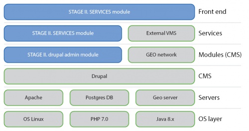
The system was hierarchically arranged in six structurally connected sets. The bottom OS layer was platform independent, meaning that STAGE II could be installed in any environment that supported Java 8; Java was needed to run the GeoServer. At the time of the study, the Postgres database was used with a Postgis add-on. Apache was used as a webserver. CMS Yii, which was used in STAGE I, was replaced by Drupal (as it was considered the latter offered a more comfortable user experience). GEO network was used as a tool to handle INSPIRE contractual obligations. External VMS services were also included to represent Open street maps and other underlying Web Map Service.
STAGE II administrative core functionalities.
- The menu tree section was used to establish a general time-independent codelist of variable names. The central part of the tab was a graphical interface designed to build a tree menu structure of individual variables as it would be displayed to the STAGE client.
- The variables section was used to import data that corresponded to a single variable defined in the menu tree. Each individual row represented a variable defined for a single spatial unit.
- Variable parameters could be set for a single variable, for a single time intersect, or for a single spatial unit. There was an option to set variable parameters for all variables that corresponded to a single menu tree entry.
- Polygons that corresponded to a single spatial unit could possibly vary over time; therefore, STAGE offered an on-the-fly table joining service when the STAGE client requested data for a choropleth map. In terms of database relations, data on geospatial layers were independent from the data on variables.
STAGE II client functionalities.
- The information page for the selected variable was directly linked to the content shown on the map. At any one time, only a single variable could be displayed on one map in one spatial layer in one time cross-section.
- In addition to the variable description, the user could choose to change the colour scheme, transparency and the classification method. Various methods of data sharing were also provided.
- A choropleth map was rendered according to instructions and the dataset stored in STAGE II administrative core. The STAGE II client was designed to offer various display settings, for example, different ways to determine the class boundaries in each map.
- All values could be displayed in a bar chart and some specific elements could be drawn in the chart. Elements could be defined using different methods: drawing points, circles, rectangles or other polygons.
Results
Geospatial statistical database on income statistics
A new database on income statistics was created. As data were only available for one relatively old reference period (2014), the data on income and poverty for lower geospatial units were not published. It is expected to publish these as a time series when more reference periods become available.
Geospatial statistical database on health statistics
A database on health statistics with 31 indicators at the level of municipalities and local administrative units was made available. It provided an important insight into many public health topics at a detailed geospatial level and the dataset was easy to access for policymakers, thereby promoting a better understanding of the health situation, raising awareness on possible public health issues and planning/promoting activities to improve health.
Downscaling methods for sample surveys
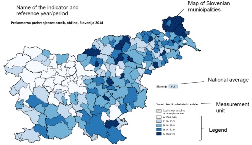
Data models were developed for downscaling methods. For each of the indicators that were modelled, point estimates were considered to be more realistic that simple estimates from survey data, especially for small municipalities. Figure 5 provides an example, showing heterogeneous variety across the country for the survey results and more homogeneous and realistic results from the modelling exercise.
Statistical confidentiality
Documentation was prepared for the record swapping method and the cell-key method.
A first set of income indicators were published for municipalities (and grid cells) after disclosure control: the median value for gross annual income; the proportion of people in the first income quintile (at a national level); the value of the first income quintile within individual municipalities; the median value of the three categories of income (from employment, pensions and benefits); the proportion of recipients for each of these three categories of income.
STAGE II
The integrated system for the dissemination of geospatial statistical data — STAGE — was upgraded in cooperation with the Geodetic Institute of Slovenia. All geospatial statistical data included in STAGE were published as free open data. The STAGE source code was made available under the European Union Public Licence.
STAGE II consists of an administrator module and a user interface. The administrator module was, among other functions, intended for: importing statistical and spatial data; hierarchical layouts; naming the displayed variables in a menu; setting visual parameters for impressions to an interactive map. The user interface was developed as a web application, the central part of which was the selected cartographic background and the overlay layer in the form of an interactive map showing statistics for the selected spatial unit. The scan menu placed to the left of the map allowed the selection of variables and dynamic time and space variations, as well as other features. A basic analysis and comparison between the displayed values was also possible.
Direct access to
Methodology
External links


