Archive:EU statistics on income and living conditions (EU-SILC) methodology – data quality

This article has been archived.

This article is part of the Eurostat online publication EU statistics on income and living conditions (EU-SILC) methodology.

Adopted in 2005, the European Statistics Code of Practice sets a number of principles for the production and dissemination of European official statistics. This constitutes comprehensive approach which builds upon a common definition of quality in statistics, in which the following dimensions are addressed: relevance, accuracy and reliability, timelines and punctuality, coherence and comparability, accessibility and clarity. This definition of quality is monitored in EU-SILC with annual quality reports prepared by both the EU Member States at national level and Eurostat at EU level. This article describes, apart from the quality reports, the following elements of EU-SILC that have an impact on the quality of data: non-sampling errors, imputation, weighting and data validation.

Full article

Non-sampling errors

The term “non-sampling error” is a generic one that encompasses any error other than sampling errors. In other terms non-sampling errors are errors that occur in all phases of the data collection and production process. Non-sampling errors are basically of 4 types:

Coverage errors: errors due to divergences existing between the target population and the sampling frame
Measurement errors: errors that occur at the time of data collection; there are a number of sources for these errors such as the survey instrument, the information system, the interviewer and the mode of data collection
Processing errors: errors in post-data-collection processes such as data entry, keying, editing and weighting
Non-response errors: errors due to an unsuccessful attempt to obtain the desired information from an eligible unit.

The non-sampling errors discussed in this section are the following: measurement errors, processing errors and non-response errors. Coverage errors are presented in the chapter about sampling.

Measurement and processing errors

Generally, measurement errors arise from the questionnaire, the interviewer, the interviewee and the data collection method used. Processing errors are mainly related to the description of data entry, coding process and the description of editing controls.

Non-response errors

There are two main types of non-response errors: unit non-response error and item non-response one. Unit non-response refers to absence of information of the whole units (households and/or persons) selected into the sample while item non-response refers to the situation where a sample unit has been successfully enumerated, but not all required information for this unit has been obtained.

Unit non-response

The Commission Regulation 28/2004 defines indicators aimed at measuring unit non-response in EU-SILC. They are respectively:

Address contact rate (Ra): the ratio of the number of addresses successfully contacted, to the number of valid addresses selected
Household response rate (Rh): the ratio of the number of household interviews completed (and accepted in the data base), to the number of eligible households at the contacted addresses
Individual response rate (Rp): the ratio of the number of personal interviews completed (and accepted in the data base), to the number of eligible individuals in completed households

Non-response is cumulative at the three stages (address contact, household interview and personal interview), so that the overall non-response rates for households and individual interviews are defined, respectively, as follows:

Overall household interview non-response rate: NRh = 1 – (Ra*Rh)
Overall personal interview non-response rate: *NRp = 1 – (Ra*Rh*Rp)

The use of models integrating external control variables is desirable in order to correct for non-response and most of the countries apply either a standard post-stratification based on homogeneous response groups or a more sophisticated logistic regression model.

Item non-response

The computation of item non-response is essential to fulfil the precision requirements. Item non-response rate is provided for the main income variables both at household and personal level and results are included in each national report. The problem of item non-response is usually dealt with imputation. It has to be kept in mind however that imputed values are not exact values and often depend on a model that could not be the perfect fit of the reality.

Imputation

There are two reasons for imputing missing data in the representative surveys such as EU-SILC; one may be referred to as statistical and the other practical. The statistical reason of imputation is to minimize error of survey estimates, in particular the non-response bias component that arises when the pattern of missing data is not random. The practical reasons concern consistency between the results from different analyses (which may handle – and be affected – differently by the problem of missing data), and the convenience of not having to deal with the missing data problem at the analysis stage.

As regards EU-SILC the imputation procedures may be applied in case of partial unit non-response or item non-response. The term “partial unit non-response” is introduced to describe the situation where not all individual members of a household selected for the survey have been successfully interviewed, while “item non-response” refers to the situation when a sample unit has been successfully enumerated, but not all the required information has been obtained.

There are different imputation techniques however all of them are based on the idea that any value (or missing value) in a sample can be replaced by a new randomly chosen value from the same source population. Imputation of missing data on a variable means replacing that missing by a value that is drawn from an estimate of the distribution of this variable. Imputation can be single or multiple. In single one, only one estimate is used. In multiple imputation, various estimates are used, reflecting the uncertainty in the estimation of this distribution. The imputation techniques can be divided into those using calculated values and those using donor method. Among the methods with calculated values are those that use calculated mean, median, trend, ratio as well as those based on linear regression. Donor based techniques are divided into those using the same source of data in order to fill in the missing information (hot deck techniques) ) and those that depend on the external data sources (cold deck techniques).

As for the imputation of missing information in EU-SILC various approaches are possible. However there are some desirable properties that the procedure should have. The Commission Regulation 1981/2003 stipulates some general rules for the imputation procedures that should be applied. According to this regulation two types of approaches (which may be used in combination) can be applied to EU-SILC data:

Imputation which makes use of the statistical relationships internal to the data set
Modelling which applies an information external to the data set

In the Regulation it is also said that the procedure applied to the data should preserve variation of and correlation between variables. Methods that incorporate “error components” into the imputed values are preferable to those that simply impute a predicted value. Additionally methods which take into account the correlation structure (or other characteristics of the joint distribution of the variables) are preferable to the marginal or univariate approach which deals with the imputation of each variable separately.

More details on the imputation methods applied by the countries conducting EU-SILC can be found in the national quality reports that can be found on Circabc.

Weighting

In the household surveys sample weights can be considered as measures of the number of persons or households the particular sample observation represents in the reference population. They are used to produce estimates of statistics that would have been obtained if the entire sampling frame had been surveyed. Sample weights allow for correcting imperfections in the sample that might lead to bias and other differences between the sample and the reference population. Such imperfections include the selection of units with unequal probabilities, non-coverage of some specific groups of population and non-response.

According to the Commission Regulation 1982/2003 on sampling and tracing rules in EU-SILC “weighting factors shall be calculated as required to take into account the units' probability of selection, non-response and, as appropriate, to adjust the sample to external data relating to the distribution of households and persons in the target population, such as by sex, age (five-year age groups), household size and composition and region (NUTS II level), or relating to income data from other national sources where the Member States concerned consider such external data to be sufficiently reliable”.

A step-by-step procedure has to be followed in order to construct correct weights in EU-SILC

Design weights Design weights are rather of methodological interest and are not used in the data analysis. They should be defined for all selected units and not only for those which respond to the survey. They are calculated by taking the inverses of the inclusion probabilities:

In case that households are sampled (or addresses or other units containing households)

Design weight = 1/(probability of selection of household)

In case that persons are sampled

Design weight = 1/∑ (probabilities of selection of eligible persons in household).

Design weights should ensure unbiased estimates for totals, however, in case of EU-SILC, because of non-response, they have to be corrected in order to reduce bias burden at the estimation stage.

Adjustments for non-response

There are different reasons for not having information collected, e.g. household refuses to cooperate or is temporarily away or data were collected but they are of insufficient quality, etc. Non-response is particularly critical when the non-responding units over-represent survey characteristics, which may create substantial bias in the estimates. Therefore good and efficient procedures to make the adjustments for non-response are very important. Unfortunately the possibilities are often constrained by lack of information as such an adjustment has to be based on characteristics which are known for both responding and non-responding units.

A classical procedure for non-response adjustment consists of modifying the design weights by a factor inversely proportional to the response rate within each weighting cell. It is common to use sampling strata or other geographical partitions as weighting cells. An alternative way to estimate response probabilities is to use a regression-based approach. Using an appropriate model such as logit regression, response propensities can be estimated as a function of auxiliary variables, which are available for both responding and non-responding units.

Adjustment to external sources – calibration

In this step weights are adjusted in order to reproduce the characteristics of the total population. Such an adjustment is called calibration. The distribution of the population e.g. by sex and age is often known from other sources such as census or population register. In case survey weights are properly adjusted, the population structure may be exactly reproduced by the sample. In EU-SILC an integrative calibration is recommended. It means both household and individual external information can be used in a single-shot calibration at household level. Individual variables are added up at household level by calculating household totals e.g. the number of males/females in the household. The calibration is then conducted at household level using household variables and the individual variables in their aggregated form. This allows using two different levels of data while keeping household and individual weights equal. It should be noted that crucial requirement in calibration is to ensure that the external control variables are strictly comparable to the corresponding survey variables, the distribution of which is being adjusted.

Trimming

It is important to ensure that no step in the weighting procedure results in extreme values of the weights, i.e. it should be ensured that large variation in the weight values is not introduced as a result of the above mentioned adjustments. Basically, at each step of the weighting procedure, the distribution of the resulting weight adjustments should be checked. There is no rigorous procedure for general use for determining the limits for trimming. While more sophisticated approaches are possible, it is recommended for EU-SILC to have a simple and practical approach.

Base weights

The base weights are computed and updated for each panel independently and that is why they are rarely used in the analysis. On the other hand they are the backbone of the computation of both cross-sectional and longitudinal weights.

For the first year wave the base weights are identical to described above adjusted design weights. In subsequent waves there will be persons leaving the target population due to different reasons e.g. due to death, migration to another country, movement out of the private household, etc. There will be also cases when the household or the person remains in the target population nevertheless the information is missing due e.g. lack of contact, refusal to participate in the country, etc. Thus the base weights at subsequent waves are the base weights from the first wave adjusted for attrition. The main difference from similar adjustment for non-response at first wave of EU-SILC is that a lot of information is available about non-respondents at subsequent waves, as those persons have been enumerated in one of the previous

Cross-sectional weights

Cross-sectional weights for the first wave are identical to the base weights described above. The following procedure describes the construction of the weights for subsequent waves.

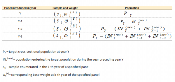
The cross-sectional sample at year Y is representative of the target cross-sectional population at Y through the selection of a sub-sample at year Y in this population. On the other hand the three preceding sub-samples do not represent new persons entering the population.

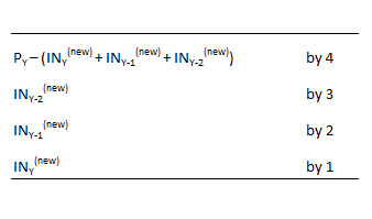
In order to put the four cross-sections together the base weights are divided in the following way:

Let ωj be the weight of unit j after the above-mentioned modification. Within a household, each member j has been assigned a weight ωj, except for "co-residents", i.e. for every household members who are ineligible for inclusion in the panel, for whom ωj=0. An average of these weights over all household members (including co-residents) is assigned to each member (including co-residents). Finally, the four panels are combined and the weights are scaled by a factor of 4:

[math]ω'_{j}=\frac{ω_{j}}{4}[/math]

The final step is to calibrate the weights against external information using the approach already described above. Integrative calibration ensures that all household members receive the same weight.

Longitudinal weights Description of longitudinal samples

If Y is the most recent year for which the data are included in EU-SILC longitudinal dataset, panels 2, 3 and 4 were selected respectively in years Y-1, Y-2 and Y-3. Thus three following longitudinal datasets of different durations are of interest:

Longitudinal set of a two-year duration, involving annual data from year (Y-1) and Y. All the three panels 2, 3 and 4, contribute to this set. In the diagram, V2 stands for the required longitudinal weight to be used in the analysis of these data. The diagram also shows the annual data sets for which this variable is required.
Longitudinal set of a three year duration, involving annual data from years (Y-2) to Y. Panels 3 and 4 contribute to this set. V3 is the required longitudinal weight for the analysis of this set. The annual data sets for which this variable is required are shown in the diagram.
Longitudinal set of a four year duration. Only panel 4 with data from years (Y-3) to Y contributes to this set. V4 is the required longitudinal weight for its analysis.

There are also other sequences of longitudinal data embedded in the data set shown in the diagram: the 3 year longitudinal sample from (Y-3) to (Y-1) in panel 4; and three 2 year samples (Y-3) to (Y-2) in panel 4, and (Y-2) to (Y-1) in panels 3 and 4.

Looking at the components of longitudinal samples (1), (2) and (3) defined above, two types can be identified:

A. Panels starting from their time of selection (t=1):

A.1.: a 2 year longitudinal sample of panel 2, covering years (Y-1) to Y

A.2: a 3 year longitudinal sample of panel 3, covering years (Y-2) to Y

A.3: a 4 year longitudinal sample of panel 4, covering years (Y-3) to Y

B. Panels which are included from a later time (t>1):

B.1: a 2 year longitudinal sample from panel 3, covering years (Y-1) to Y

B.2: a 2 year longitudinal sample from panel 4, covering years (Y-1) to Y

B.3: a 3 year longitudinal sample from panel 4, covering years (Y-2) to Y

Construction of longitudinal weights

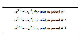
In all cases of type A above, the weights involved are identical to base weights defined earlier:

In cases B there are samples of two and three year duration. The weights for them are constructed in the following way:

Longitudinal set of two year duration for the most recent period (Y-1) to Y

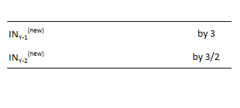
To ensure proper representation of the special groups identified in the final column the weights should be multiplied in the following way:

Then the required weights are computed as follows:

[math]V2_{j}=\frac{ω_{j}}{3}[/math]

where ω is the weight for any unit j as defined above.

Longitudinal set of three year duration (Y-2) to Y

After multiplying the weights assigned to cases in IN_Y-2^(new) by 2, the required weight for the longitudinal units of interest is computed as:

[math]V3_{j}=\frac{ω_{j}}{2}[/math]

More details about the construction of EU-SILC weights can be found in:

EU-SILC methodological guidelines DOC65

Cross-sectional and longitudinal weighting for the EU-SILC rotational design

Data Validation

There is a comprehensive validation procedure applied for EU-SILC data. All countries conducting the survey validate data before sending it to Eurostat. Countries may apply their own validation procedures in the course of data processing, nevertheless at the end of data validation at national level they should carry out the complete checking procedurethat is also applied at Eurostat. This procedure is very accurate and controls many aspects of data. It checks for syntax and logical errors, controls the weights, compares year to year results, detects outliers, etc. Along with data countries are obliged to provide to Eurostat a commented summary of the error report produced by this checking tool.

Quality Reports

The production of the quality reports is part of the implementation of the EU-SILC instrument. There are two types of the quality reports: national ones prepared by the Member States and EU ones prepared by Eurostat. The national quality reports provide useful insight into national implementation, they focus in particular on the entire statistical process, sampling and non-sampling errors and potential deviations from standard definitions and concepts. The purpose of the EU quality reports is to summarize the information contained in the national quality reports. Their objective is to evaluate the quality of EU-SILC data from a European perspective, i.e. by establishing cross-country comparisons of some of its key quality characteristics. The EU quality reports, as well as most of the national reports, are publicly available on Circabc.

The Commission Regulation 28/2004 describes the content of the intermediate and final quality reports, however the current content of the quality reports does not fully reflect the template stated there. This is due to the fact that the European Statistical System (ESS) has established a common standard for the quality reports structure (ESS Standard for Quality Reports Structure - ESQRS) that should be introduced whenever the quality of data is reported. The main concepts used by ESQRS are the following: assessment of the quality management, relevance, accuracy and reliability, timeliness and punctuality, accessibility and clarity, comparability, coherence, cost and burden, confidentiality and statistical processing. More about EU standards for quality reporting can be found in ESS Handbook for quality reports.