Archive:EU statistics on income and living conditions (EU-SILC) methodology – concepts and contents

This article has been archived.

This article is part of a set of articles presenting the variables that the European Union's (EU) Member States compile and transmit to Eurostat in the frame of EU-SILC survey as well as all variables included in the ad-hoc modules. The article also describes the methodology applied by Eurostat for the computation of additional variables used to ease further statistical computations.

The approach followed for the presentation of the variables involved in the production process of EU-SILC statistics is based on their relationship to the statistical units of the survey. In EU-SILC, private households - collective households and institutions are excluded from target population - form the basic units of sampling and data collection, while information that pertains to individual persons is also directly collected from them. In terms of the statistical units, two types of variables measured and analyzed are thus involved in EU-SILC: variables (a) at household level and (b) at personal level. These “target variables” are either compiled from registers (register variables), or collected from the sampled units (observation variables).

On the basis of these target variables, additional variables (derived variables) are calculated for each statistical unit-observation, to support the computation of the indicators. Additionally, a relatively important component of the variables is the linking or identification variables, such as the year of the survey, that characterize the whole survey. Auxiliary variables on the other hand, are also computed variables but rather than referring to distinct statistical units-observations, they refer to the whole statistical population. These include statistical measures, thresholds, etc.

Full article

Household variables

Household variables refer to the set of variables (either collected or computed) that concern the household. These variables may be collected or derived from both cross-sectional and longitudinal components of EU-SILC.

Household register variables

Household register variables are variables that concern the household per se. The household register variables compiled by the Member States are listed below.

• Region (DB040)
• Degree of urbanisation (DB100)

More detailed description of the variables is provided in the Methodological guidelines and description of EU-SILC target variables.

Table 1: Household observation variables

Household observation variables

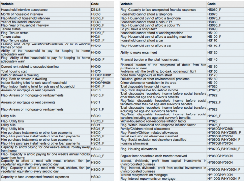
Household observation variables are variables collected from the sampled units and concern the household in relation with the observed phenomenon. These variables are listed in Table 1 and are described in detail in the Methodological guidelines and description of EU-SILC target variables.

Household derived variables

The household derived variables are additional computed variables concerning the statistical unit, i.e. the household, and are calculated in order to support further computations. These variables are calculated by Eurostat based on the micro-data received by the Member States and further used for the computation of the indicators and dimensions along with the indicators are disseminated. The process for their calculation is described for each variable separately and is derived on the basis on the corpus of SAS scripts.

The list of variables calculated by Eurostat is presented below, along with the description for their computation.

Degree of urbanisation (DEG_URB)

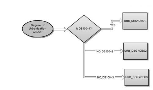
The degree of urbanisation of the area where the respondent’s household belongs is recorded in the basic SILC variable DB100. The following degrees of urbanisation are considered:

• DEG1 (Densely populated area: At least 50 % lives in contiguous grid cells of 1k² with a density of at least 1 500 inhabitants per k² and a minimum population of 50 000)
• DEG2 (Intermediate density area: Clusters of contiguous grid cells of 1k² with a density of at least 300 inhabitants per k² and a minimum population of 5 000)
• DEG3 (Thinly-populated area: More than 50 % of the population lives in rural grid cells outside urban clusters)

The above degrees of urbanisation categories using the variable DB100 are defined as shown below:

Equivalised Disposable Income (EQ_INC)

Equivalised disposable income (EQ INC) is the total income of a household that is available for spending or saving, divided by the number of household members converted into equivalised adults; household members are equivalised or made equivalent by the following so-called modified OECD (Organisation for Economic Co-operation and Development) equivalence scale:

• the first household member aged 14 years or more counts as 1 person
• each other household member aged 14 years or more counts as 0.5 person
• each household member aged 13 years or less counts as 0.3 person

The algorithm for equivalised disposable income uses the following auxiliary variables:

• PY80 - Pension from individuals private plans (constructed)
• SUM_PY80 - The sum of pensions from individuals private plans at household level before 2009 (constructed)
• SUM_PY080G - The sum of pensions from individuals private plans at household level after 2008 (constructed)
• EQ_SS - Equivalised household size (constructed)

The calculation of variables PY80, SUM_PY80 and SUM_PY080G are described below.

i) PY80

PY80

ii) SUM_PY80 The sum of pensions from individuals private plans at household level for years before 2009 is recorded in variable SUM_PY80 and is calculated as follows:

if DB010<2009 then [math]SUM\_PY80=\sum\limits_{i}{PY80}[/math]

iii) SUM_PY080G The sum of pensions from individuals private plans at household level for years after 2008 is recorded in variable SUM_PY080G and is calculated as follows:

if DB010>2008 then [math]SUM\_PY080G=\sum\limits_{i}{PY080G}[/math]

The Equivalised disposable income calculation (EQ_INC20, EQ_INC22, EQ_INC23) is described below.

a) Equivalised disposable income after social transfers (EQ_INC20)

if DB010>2008 then [math]EQ\_INC20=\frac{(HY020+SUM\_PY080G)\times\;HY025}{EQ\_SS}[/math]

if DB010<2009 then [math]EQ\_INC20=\frac{(HY020+SUM\_PY80)\times\;HY025}{EQ\_SS}[/math]

b) Equivalised disposable income before social transfers (excluding old-age and survivor’s benefits/pensions) (EQ_INC22)

if DB010>2008 then [math]EQ\_INC22=\frac{(HY022+SUM\_PY080G)\times\;HY025}{EQ\_SS}[/math]

if DB010<2009 then [math]EQ\_INC22=\frac{(HY022+SUM\_PY80)\times\;HY025}{EQ\_SS}[/math]

c) Equivalised disposable income before social transfers (including old-age and survivor’s benefits/pensions) (EQ_INC23)

if DB010>2008 then [math]EQ\_INC23=\frac{(HY023+SUM\_PY080G)\times\;HY025}{EQ\_SS}[/math]

if DB010<2009 then [math]EQ\_INC23=\frac{(HY023+SUM\_PY80)\times\;HY025}{EQ\_SS}[/math]

In the above calculations we make use of the Equivalised household size (EQ_SS).

Note: All calculations have been made in both Euros (Euro (from 1.1.1999)/ECU (up to 31.12.1998)) and PPP.

→ SAS program: VAR_HY20_EQ_INCXX.sas, idb_calculation.sas, VAR_EQ_SS.sas

Equivalised household size (EQ_SS)

The algorithm for equivalised household size uses the following auxiliary variables:

• hm13 - Number of household members aged 13 or less
• hm14 - Number of household members aged 14 and over
• SUM_hm13 - The total number of household members (at household level) with age 13 or less
• SUM_hm14 - The total number of household members (at household level) with age 14 and over

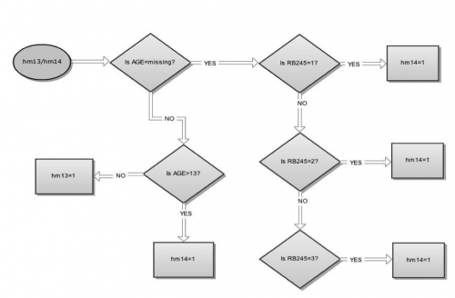
The calculation of variables hm13 and hm14 are described schematically below:

→ SAS program: idb_calculation.sas, VAR_EQ_SS.sas

Household cost burden (HCB)

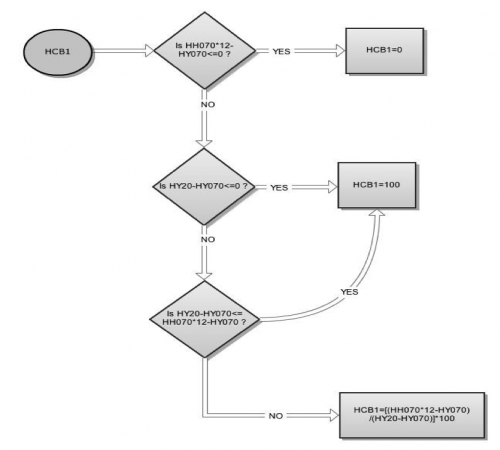
Household cost burden variable (HCB) definition uses the auxiliary variables HCB1, HY20, HY070; their definition is presented schematically below:

a. Total disposable household income including pension from individual private plans (HY20): [math]HY20=EQ\_INC20*EQ\_SS[/math]

where Equivalised Disposable Income (EQ_INC) and Equivalised Household Size (EQ_SS) have already been presented

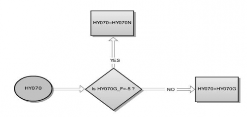
b. Housing allowances - HY070:

c. Household cost burden threshold - HCB1:

The HCB threshold was set at 40 % of the total disposable household income. So the variable household cost burden (HCB) is defined as follows:

[math]if \;\;HCB1\gt 40\;\;then\;\;HCB1=1[/math]

[math]if \;\;HCB1\leq 40\;\;then\;\;HCB1=0[/math]

→ SAS program: lvh07.sas, VAR_HY20_EQ_INCXX.sas

Household type (HHTYP)

The following household types will be considered:

• TOTAL Total (HHTYP=1-13)
• A1 Single Person (HHTYP=1-5)
• A1_LT65 One adult younger than 65 (HHTYP=1,2)
• A1_GE65 One adult older than 65 (HHTYP=3,4)
• A1_DCH Single person with dependent children (HHTYP=9)
• A1M Single male (HHTYPE=1,3)
• A1F Single female (HHTYP=2,4)
• A2 Two adults (HHTYP=6,7)
• A2_2LT65 Two adults, no dependent children, younger than 65 years (HHTYP=6)
• A2_GE1_GE65 Two adults, no dependent children, at least one adult 65 years or more (HHTYP=7)
• A2_1DCH Two adults with one dependent child (HHTYP=10)
• A2_2DCH Two adults with two dependent children (HHTYP=11)
• A2_GE3DCH Two adults with three or more dependent children (HHTYP=12)
• A_GE2_NDCH Two or more adults without dependent children (HHTYP=6-8)
• A_GE2_DCH Two or more adults with dependent children (HHTYP=10-13)
• A_GE3 Three or more adults, no dependent children (HHTYP=8)
• A_GE3_DCH Three or more adults with dependent children (HHTYP=13)
• HH_NDCH Households without dependent children (HHTYP=1-8)
• HH_DCH Households with dependent children (HHTYP=9-13)
• UNK Others (not possible to determine type) (HHTYP=16)

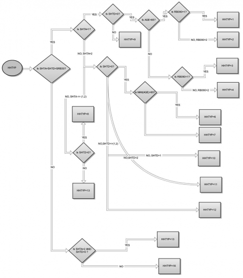
The calculation of the household type variable for the respondent uses the following auxiliary variables.

• HT_D - Number of dependent children in the household
• HT_A - Number of adults in the household
• SHTD - Total number of dependent children in the household
• SHTA - Total number of adults in the household
• SRB30 - The number of Personal IDs (RB030)

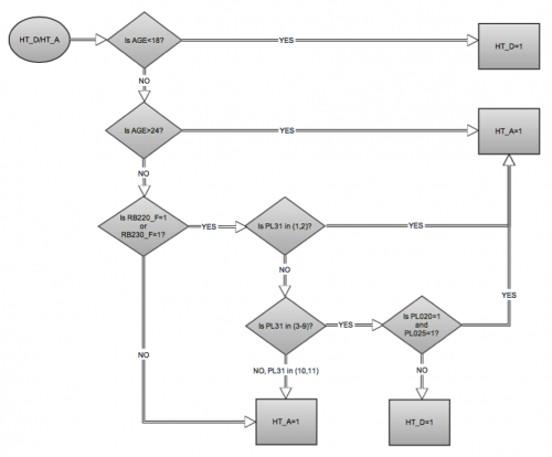
The calculation of the household type variable (HHTYP) for the respondent depends on the concepts of the adult and dependent child. Below the algorithm dividing respondents to adults or dependent children is described graphically. The variables HT_D and HT_A are used to define a respondent as dependent child or an adult respectively.

The variables HT_D and HT_A are used to derive the auxiliary variables SHTD (SHTD=sum (HT_D)) and SHTA (SHTA=sum (HT_A)), which describe the total number of dependent children and the total number of adults in household level. These auxiliary variables are used for the calculation of the variable household type (HHTYP):

→ SAS program: VAR_HT_NADU_NDCH.sas, VAR_HT1.sas

Household type (children living with parents)

The following household types will be considered:

1. Child living in a household with both parents cohabiting
2. Child living in a household with both parents married
3. Child living in a household with a single parent
4. Child not living with parents

The calculation of the household type variable for the respondent uses six auxiliary variables. The four of which come from EU - SILC:

• F_PB180 - Father spouse/partner ID
• F_PB030 - Father personal ID
• M_PB180 - Mother spouse/partner ID
• M_PB180 - Mother spouse/partner ID

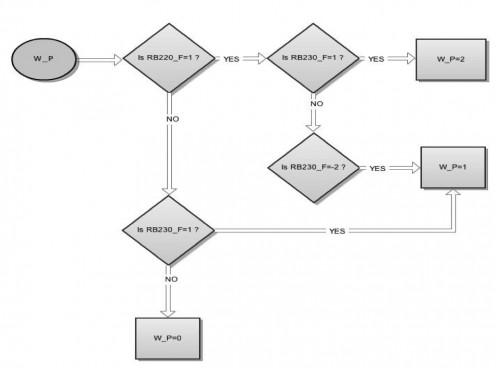
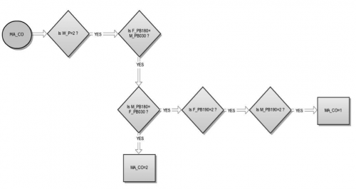
The other two variables of W_P (indicator showing the number of parents living in the household) and MA_CO (indicator showing whether the parents living in the household are married) have been constructed.

The calculation of the household type variable (HHTYP2) for the respondent depends on the above auxiliary variables W_P and MA_CO. Below we describe graphically the algorithm calculating the auxiliary variables:

a. W_P

b. MA_CO

The calculation of the household type variable (HHTYP2) is described graphically below:

→ SAS program: _lvps20.sas, _lvps30.sas

Income quantile

Dividing ordered data into q essentially equal-sized data subsets is the motivation for q – quantiles; the q – quantiles are the data values marking the boundaries between consecutive subsets. Put another way, the k^th q – quantile for a random variable is the value x such that the probability that the random variable will be less than x is at most [math]\frac{k}{q}[/math] and the probability that the random variable will be more than x is at most [math]\frac{q-k}{q}=1-\frac{k}{q}[/math]. There are q of the q – quantiles, one for each integer k satisfying [math]0\lt k\leq q[/math].

For some q – quantiles there are special names:

• The 2 – quantile is called the median
• The 3 – quantiles are called tertiles
• The 4 – quantiles are called quartiles
• The 5 – quantiles are called quintiles
• The 10 – quantiles are called deciles
• The 100 – quantiles are called percentiles

Below we describe the calculation of the q – quantile interval which a person belongs to. A person belongs to the 1^st q – quantile if his/her equivalised disposable income is less than or equal to the equivalised disposable income of the person with the highest equivalised disposable income within the [math]\frac{1}{q}\times100\%[/math] of people which have the least income.

A person belongs to the k^th q – quantile [math](0\lt k\leq q)[/math] if his/her equivalised disposable income is:

• less than or equal to the equivalised disposable income of the person with the highest equivalised disposable income within the [math]\frac{1}{q}\times100\%[/math] of people which have the least income, and
• higher than the equivalised disposable income of people in [math]\frac{k-1}{q}\times100\%[/math] of the population the lowest equivalised income.

The procedure for calculating the q – quantile where a person belongs is broadly similar to the procedure applied for the calculation of the median (i.e. persons will be sorted according to their equivalised disposable income (sorting order: lowest to the highest value)), but here the cut-off points will be:

[math]Cut-off-point_i=\frac{k}{q}\times100\%\times\sum \limits_{i=1}^{n}RB050a_i[/math]

Where:

n = number of persons (household members)

RB050ai = is the Adjusted cross sectional weight (RB050a)

for person i and k an integer satisfying the condition

The k^th q – quantile equivalised disposable income [math]EQ\_INC_{at\_k\_q\_quantile}[/math] giving the disposable income in the k^th q – quantile interval is calculated as:

[math]EQ\_INC_{at\_k\_q\_quantile}=\left\{\begin{matrix} \frac{1}{2} (EQ\_INC20_j+EQ\_INC_{j+1}),\;if\;\sum\limits_{i=1}^{j}RB050a_i=\frac{k}{q}\times\;100 \%\;\sum\limits_{i=1}^{n}RB050a_i\\ EQ\_INC20_{j+1},\;if\;\sum\limits_{i=1}^{j}RB050a_i\lt \frac{k}{q}\times\;100\%\sum\limits_{i=1}^{n}RB050a_i\lt \sum\limits_{i=1}^{j+1}RB050a_i \end{matrix}\right.[/math]

Where: EQ_INC20i is the Equivalised disposable Income (EQ_INC) (after social transfers) of person i,

RB050ai is the Adjusted cross sectional weight (RB050a) for person i,

n is the number of persons (household members) and

k is an integer satisfying the condition.

Persons have to be sorted according to their Equivalised disposable Income (EQ_INC) (after social transfers) (sorting order: lowest to highest value, household identification number and personal identification number).

→ SAS program: VAR_QITILE.sas

Lack of bath or shower (LACK_BS)

This variable refers to the lack of bath or shower, which is related to the basic EU-SILC variables HH080 and HH081. For the calculation of variable is also used the flag of EU – SILC variable HH081 (HH081_F). The calculation of variable LACK_BS is presented schematically below:

→ SAS program: mdho06.sas, mdho02.sas

Lack of bath or shower and lack of toilet (LACK_BSΤ)

This variable refers to the lack of bath or shower and the lack of indoor flushing toilet for sole use of household toilet, which is related to the basic EU-SILC variables HH080, HH081, HH090 and HH091. For the calculation of variable are used the derived variables Lack of toilet (LACK_TOILET) and Lack of bath or shower (LACK_BS). The calculation of variable LACK_BST is presented below:

[math]LACK\_BST=\left\{\begin{matrix} 1\;if\;LACK\_TOILET=1\;and\;LACK\_BS=1 \\ missing,\;if \;LACK\_TOILET\;missing\;or\;LACK\_BS\;missing \end{matrix}\right. [/math]

→ SAS program: mdho06.sas, mdho05.sas

Lack of toilet (LACK_TOILET)

This variable refers to the lack of indoor flushing toilet for sole use of household, which is related to the basic EU-SILC variables HH090 and HH091. For the calculation of variable LACK_TOILET the flag of EU – SILC variable HH091 (HH091_F) is also used . The calculation of variable is shown schematically below:

→ SAS program: mdho06.sas, mdho03.sas

Material deprivation (MD)

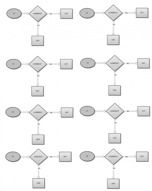
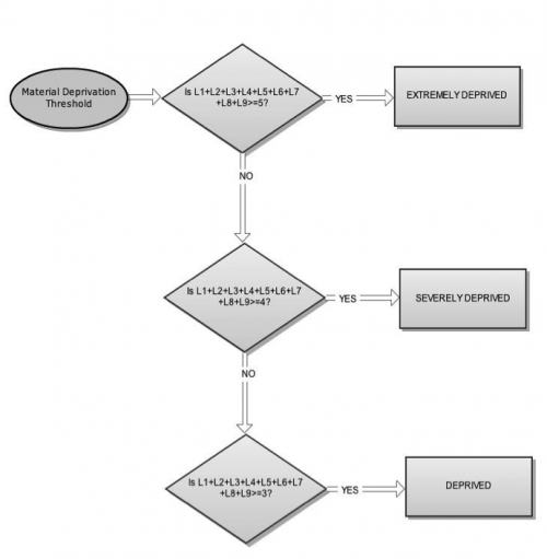
The material deprivation rate refers to the situation of people who cannot afford a number of necessities considered essential to live a decent life in tion items. The nine material deprivation items considered are:

• L1-Arrears on mortgage or rent payments (basic variable HS010/HS011), utility bills (basic variable HS020/HS021), hire purchase instalments or other loan payments (basic variable HS030/HS031)

• L2-Capacity to afford paying for one week’s annual holiday away from home (basic variable HS040)
• L3-Capacity to afford a meal with meat, chicken, fish (or vegetarian equivalent) every second day (basic variable HS050)
• L4-Capacity to face unexpected financial expenses (basic variable HS060)
• L5-Household cannot afford a telephone (including mobile phone) (basic variable HS070)
• L6-Household cannot afford a colour TV (basic variable HS080)
• L7-Household cannot afford a washing machine (basic variable HS100)
• L8-Household cannot afford a car (basic variable HS110)
• L9-Ability of the household to pay for keeping its home adequately warm (basic variable HH050)

Individuals are considered deprived if they have an enforced lack of at least three out of nine material deprivation items. The calculation of materially deprivation rate using the nine families of material deprivation items is presented below:

→ SAS program: VAR_DEP_SEV_EXT_Reliability.sas

Number of children (NUM_OF_CHLD)

The number of children variable is concerned with the definition of the total number of children (people aged less than 18 years) living in the household. For the calculation of the number of children variable is used the auxiliary variable child defined with the help of the derived variable Age as follows:

[math]Child\;=\left\{\begin{matrix} 1,\;if\;Age\lt 18 \\ 0,\; if\;Age\geq 18 \end{matrix}\right.[/math]

So the number of children living in a household equal to:

[math]NUM\_OF\_CHLD=\sum\limits_{i=1}^{n}Child_i[/math]

where [math]n[/math] corresponds to the total number of persons living in the household.

→ SAS program: _lvph05.sas

Nuts region

The respondent’s region of residence is recorded in the basic SILC variable DB040; this variable helps for the calculation of the NUTS region variable. There are two levels of aggregation for the variable NUTS, the NUTS1 level and the NUTS2 level. The calculation of the NUTS variables using the basic SILC variable is as follows:

[math]NUTS2\;=DB040[/math]

[math]NUTS1\;the\_first\_three\_characters\_of\_DB040[/math]

Overcrowding and Under-occupation

The calculation algorithm for the variables overcrowding and under-occupation uses the auxiliary variables presented below:

• ADULT_PARTNER - Persons living in a couple
• ADULT_SINGLE - Adults not living in a couple
• CHILD_LESS_12 - Children at age of 0-11
• TEENAGE_MALE - Boys at the age of 12-17
• TEENAGE_FEMALE - Girls at the age of 12-17
• COUPLE_ROOM - The minimum necessary rooms for the couples (one room per couple)
• ADULT_SINGLE_ROOM - The minimum necessary rooms for single adults (one room per adult)
• CHILD_ROOM - The minimum necessary rooms for children at age 0-11 (one room per pair of children)
• TEEN_MALE_ROOM - The minimum necessary rooms for boys at age 12-17 (one room per pair of boys)
• TEEN_FEMALE_ROOM - The minimum necessary rooms for girls at age 12-17 (one room per pair of girls)

The definition of the above described auxiliary variables, with the help of the derived variable Age, is presented schematically below:

The next step for the calculation of the variables overcrowding and under-occupation is to estimate the number of rooms for each household based on the following rules:

• One room for the household
• One room for each couple in the household
• One room for each single person aged 18 and over
• One room for two single people of the same sex between 12 and 17 years of age
• One room for each single person of different sex between 12 and 17 years of age
• One room for two people under 12 years of age

The number of different type rooms for each household is calculated below:

Couple Room: [math]\; COUPLE \_ROOM = CEIL\left ( \frac{ \sum ADULT\_ \:PARTNER}{2} \right )[/math]

Adult single Room: [math]\; ADULT \_SINGLE\_ROOM = {\sum ADULT\_ \, SINGLE}[/math]

Child Room: [math]\; CHILD \_ ROOM = CEIL\left ( \frac{ \sum CHILD\_ \, LESS\_\,12}{2} \right )[/math]

Teen Male Room: [math]\; TEEN \_ MALE\_ROOM = CEIL\left ( \frac{\sum TEENAGE\_ \, MALE}{2} \right )[/math]

Teen Female Room: [math]\; TEEN \_FEMALE\_ROOM = CEIL\left ( \frac{\sum TEENAGE\_ \, FEMALE}{2} \right )[/math]

Finally, if the household does not have at its disposal a minimum number of rooms considered adequate, it is defined as overcrowded. The overcrowding variable is calculated as shown schematically below:

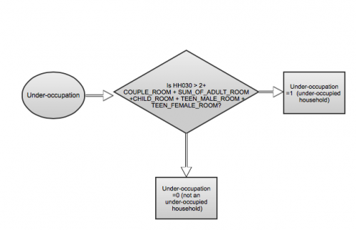
Additionally, if the household has at its disposal more than the minimum number of rooms considered adequate, it is defined as under-occupied. The under-occupation variable is calculated as shown schematically below:

→ SAS program: VAR_OVERCROWDED.sas, lvho50.sas

Pension income (INCPEN)

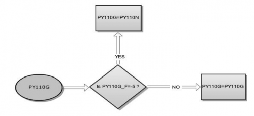
The income from pensions variable (INCPEN) is defined as: [math]INCPEN\;=\;PY80\;+\;PY100G\;+\;PY110G[/math]

The flags of the above variables (PY080G_F, PY100G_F, PY110G_F) are used to define the relevant variables:

→ SAS program: VAR_INCWRK_INCPEN.sas

Poverty status (ARPTXXi)

The risk of poverty indicator identifies people below the At-risk-of-poverty threshold (ARPTXX) (ARPT60i=1) from people with Equivalised Disposable Income (EQ_INC) after social transfers (EQ_INC20) above the risk of poverty threshold (ARPT60i=0).

if EQ_INC20<ARPT then ARPTXXi=1

if EQ_INC20>=ARPT then ARPTXXi=0

The usual definition defines at-risk-of-poverty threshold as 60% of the equivalised median income so the value of variable XX in the usual definition is 60 (ARPT60i).

Self-defined working status (SELF_WSTATUS)

The self – defined working status is the status that individuals declare themselves as their main activity at present. The following working statuses will be considered:

a. Employees with a permanent job

b. Emploees with a temporary job

c. Employed persons except employees

d. Unemployed persons

e. Students

f. Retired persons

g. Other inactive persons

The calculation of the self – defined working status variable for the respondent uses the following auxiliary variables.

• PL31 - Variable showing the self – defined current economic status with 9 categories instead of the 11 categories of the initial variable PL031 (Adjusted self – defined current economic status (PL31)) (constructed)
• PL040 - Status in employment (EU-SILC)
• PL140 - Type of contract (EU-SILC)

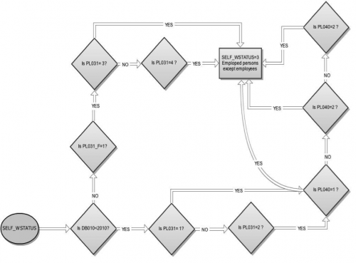
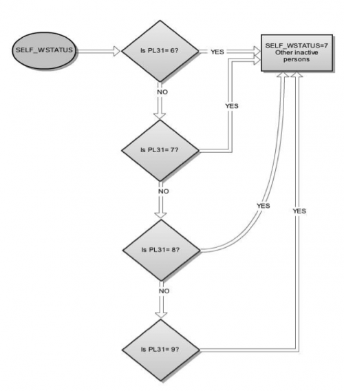
The calculation of the self – defined working status variable (SELF_WSTATUS) for the respondent for each working status is described graphically below.

a. Employees with a permanent job

b. Emploees with a temporary job

c. Employed persons except employees

d. Unemployed persons

e. Students

f. Retired persons

g. Other inactive persons

Note: The flow charts deiscribing the calculating algorithms for self – defined working statuses considered above of the derived variable Adjusted self – defined current economic status (PL31).

→ SAS program: L_lvhl33.sas

Severe housing deprivation (SEV_HH_DEP)

Severe housing deprivation refers to people living in an overcrowded dwelling deprived by at least one housing deprivation item. The housing deprivation items considered, along with their calculation formula, are:

• Leaking roof, damp walls/floors/foundation, or rot in window frames or floor (HH040): [math]LEAKING\_ROOF=\left\{\begin{matrix} 1,\;if\;HH040=1\\ 0,\;if\;HH040=2 \end{matrix}\right.[/math]

• No bath or shower in the dwelling (HH080, HH081) and no indoor flushing toilet for the sole use of the household (HH090, HH091): Lack_of_bath_or_shower_and_lack_of_toilet_(LACK_BST), Lack of toilet (LACK_TOILET).

• Dwelling too dark (HS160): [math]TOO\_DARK=\left\{\begin{matrix} 1,\;if\;HS160=1\\ 0,\;if\;HS160=2 \end{matrix}\right.[/math]

• Overcrowding

So, Severe housing deprivation is equal to:

[math]SEV\_HH\_DEP=\left\{\begin{matrix} 1,\;if\;OVERCROWDING=1\;and(LEAKING\_ROOF=1\;or\;TOO\_DARK=1\;or\;LACK\_BST=1) \\ missing,\;if\;OVERCORWDING\;is\;missing \end{matrix}\right.[/math]

→ SAS program: mdho06.sas

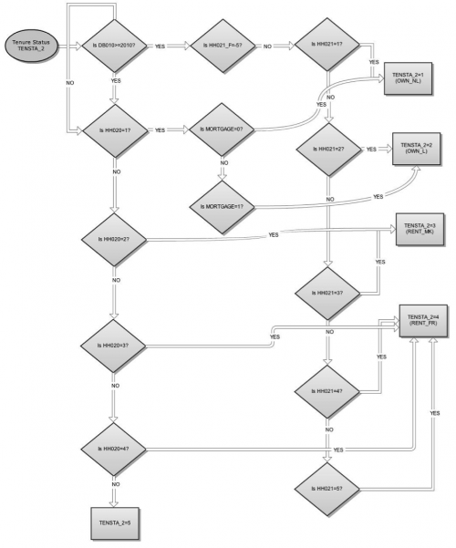
Tenure status (TENSTA_2)

The following accommodation tenure statuses will be considered:

• OWN - Owner
• OWN_L - Owner, with mortgage or loan
• OWN_NL - Owner, no outstanding mortgage or housing loan
• RENT - Tenant
• RENT_MKT - Tenant, rent at market price
• RENT_FR - Tenant at reduced price or free
• TOTAL - Total

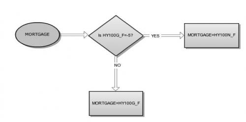
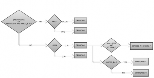
The calculation algorithm for variable accommodation tenure status uses the auxiliary variable mortgage defined as follows:

The definition of variable accommodation tenure status is shown below schematically:

→ SAS program: VAR_TENSTA_2.sas

Tenure status (TENSTA)

The following accommodation tenure statuses will be considered:

• OWN - Owner
• RENT - Tenant

The calculation algorithm for variable accommodation tenure status uses the auxiliary variable mortgage defined as follows:

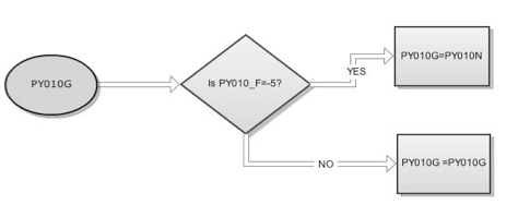
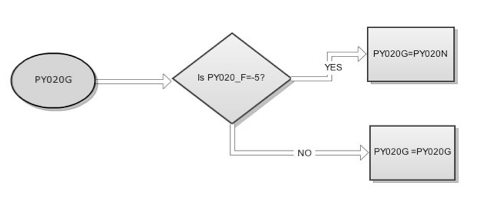
Working income (INCWRK)

The income from work variable (INCWRK) is defined as:

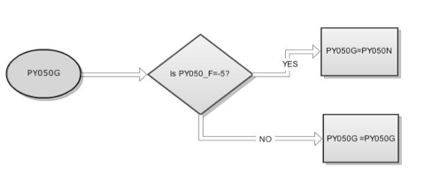
[math]INCWRK=PY010G+PY020G+PY050G[/math]

The flags of the above variables (PY010G_F, PY020G_F, PY050G_F) are used to define the relevant variables:

→ SAS program: VAR_INCWRK_INCPEN.sas

Work intensity (WI)

The work intensity of the household refers to the number of months that all working age household members have been working during the income reference year as a proportion of the total number of months that could theoretically be worked within the household.

A working age is defined as a person aged 18-59, not being a dependent child. Dependent children include all persons aged below 18 as well as persons aged 18 to 24 years, living with at least one parent and economically inactive (see variable Household type (HHTYP)). The calculation algorithm for the working intensity uses the following auxiliary variables:

• Hourx/Hourx2 - Total hours worked per week (constructed)
• C_mean - The mean of working hours of those who work part-time at the time of interview (constructed)
• Houratio - An estimation of part-time ratio (constructed)
• NW - Total number of workable months (constructed)
• Ne1/Ne2 - Total number of months actually worked (constructed)
• Imputedone - Flag that indicates if a record is corrected for non-response (using HY025 variable)
• Imputetodo - Flag that points records that have to be corrected after the application of the HY025 variable
• Imputetodohh - Flag that points the total number of records that have to be corrected after the application of the HY025 variable at household level
• Monthratio - An estimation of the part of the year actually worked by the respondent (constructed)
• wi - The sum of month ratios of all working age members of a household (constructed)
• Size - The number of working age members of a household (constructed)
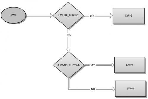
• WORK_INT - Household work intensity expressed as the average month ratio for a household (only working age household members are included) (constructed)
• LWI - Low work intensity flag

The starting point of work intensity algorithm is the calculation of the total number of hours worked per week (hourx/hourx2) for each respondent. The calculation of auxiliary variables hourx and hourx2 is presented schematically below:

An estimation of the part-time hours ratio is needed in order to equivalise full time and part- time hours worked by the working age members of the household in order.

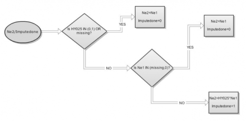
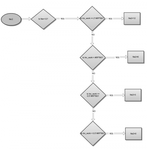
The calculation of the total equivalised months actually worked (Ne1) as well as the total number of workable months (Nw) for the working age members of the household is presented schematically below:

The calculation of the total equivalised months actually worked corrected for non-response (Ne2) is presented schematically below:

For the problematic case where the basic SILC variables used for the calculation of the total number of workable months (PL073-PL090) are missing, the auxiliary variable Ne2 is calculated using the:

Working Income (INCWRK) at individual level. The calculation of variable Ne2 is shown schematically below:

Especially for years before 2009 in order to solve the problem of full P-record missing for all working age members of the household, it is used the income information (Equivalised disposable Income (EQ_INC) before social transfers EQ_INC22) at the household level for the calculation of the Ne2 variable. More specifically:

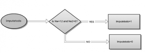
To detect the records still need imputation at the household level we form the flag imputetodo. The calculation of flag imputetodo is presented below:

An estimation of the part of the year actually worked by each member of the household at working age can be calculated as described below:

[math]month\_ratio=\frac{Ne2}{12}[/math]

The sum of month ratios for all household members at working age define auxiliary variable wi:

[math]wi=\sum\limits_{i}{month\_ration\_i},\;\;\;\;i\in [1,size][/math]

In the above definition the auxiliary variable size express the total number of household members at working age and defined as:

[math]size=\sum{RB030}[/math]

The variable swi has to correct for the problematic cases where the full P-record missing for all working age members of the household, the correction of variable swi it is based on the income information (disposable income before social transfers EQ_INC22) at the household level. More specifically:

Finally the work intensity variable defined as [math]WORK\_INT=\frac{wi}{size}[/math]

[math]if\; WORK\_INT\gt 1\;\;then\;\;WORK\_INT= 1[/math]

[math]if\; Age\gt 59\;\;then\;\;WORK\_INT= 99[/math]

[math]if\; WORK\_INT=missing\;\;then\;\;WORK\_INT= 99[/math]

The work intensity variable is also used to calculate the low work intensity variable (LWI) as:

→ SAS program: VAR_LWI_WORK_INT.sas

Person variables

Person variables refer to the set of variables (either collected or computed) that concern the person. These variables may be collected or derived from both cross-sectional and longitudinal components of EU-SILC.

Person register variables

Table 2: Person observation variables

Person register variables are variables that concern the person per se. The person register variables compiled by the Member States are listed below.

• Sex (PB150)
• Spouse/partner ID (PB180)
• Country of birth (PB210)
• Citizenship (PB220A)

More detailed description of the variables is provided in the Methodological guidelines and description of EU-SILC target variables.

Person observation variables

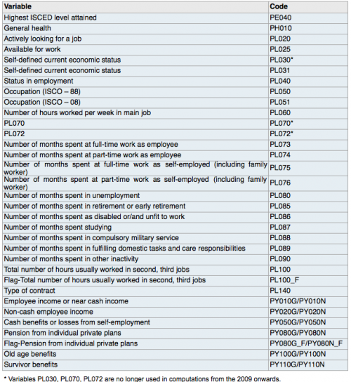
Person observation variables are variables collected from the sampled units and concern the person in relation with the observed phenomenon. These variables are listed in Table 2 and are described in detail in the Methodological guidelines and description of EU-SILC target variables.

Person derived variables

The person derived variables are additional computed variables concerning the statistical unit, i.e. the person, and are calculated in order to support further computations. These variables are calculated either by the Member States or by Eurostat based on the micro-data received by the Member States. This set variables is used in the computations of the indicators and dimensions along with the indicators are disseminated. The process followed by Eurostat for their calculation is described for each variable separately and is derived on the basis on the corpus of SAS scripts.

The list of person derived variables that are computed by the Member states is the following:

• Personal cross-sectional weight (PB040)
• Personal base weight for selected respondent (PB080)
• Cross sectional weight (RB050)
• Personal base weight (RB060)
• Longitudinal weight (two – year duration) (RB062)
• Longitudinal weight (three – year duration) (RB063)
• Longitudinal weight (four – year duration) (RB064)

Further information about these variables and their compilation is provided in the Methodological guidelines and description of EU-SILC target variables.

The list of variables calculated by Eurostat is presented below, along with the description for their computation.

Activity Status (ACTSTA)

For each household member aged 16 and over, the number of months in each status during the income reference period is counted. The following activity statuses will be considered: TOT - Total number of months spent in any status during the reference period

POP - Total population

EMP - Number of months spent in work for employed persons

SAL - Number of months spent in work for employees

NSAL - Number of months spent in work for employed persons except employees

UNEMP - Number of months spent in unemployment

RET - Number of months spent in retirement

INAC_OTH - Number of months spent as ‘other inactive’ (in education or training, doing housework, looking after children or other persons; in community or military service; other economically inactive)

The calculation of the current activity status of the respondent depends on the year of survey and more specifically if it is before or after 2008.

• For surveys after 2008 (DB010>2008)

For each household member the following variables will be selected: PL073, PL074, PL075, PL076, PL080, PL085, PL086, PL087, PL088, PL089, PL090. The following derived variables will be constructed:

TOT= PL073+PL074+PL075+PL076+PL080+PL085+PL086+PL087+PL088+PL089+PL090

SAL= PL073+PL074

NSAL= PL075+PL076

UNEMP= PL080

RET= PL085

INAC_OTH= PL086+PL087+PL088+PL089+PL090

The respondent is being excluded if the total number of months spent in any activity is less than seven (TOT<7). For the rest of the respondents that have reported for more than six months the activity status is calculated as follows:

[math]if \;\;\frac{EMP}{TOT}\gt 0.5[/math] then Activity status=1

[math]if \;\;\frac{UNEMP}{TOT}\gt 0.5[/math] then Activity status=5

[math]if \;\;\frac{RET}{TOT}\gt 0.5[/math] then Activity status=6

[math]if \;\;\frac{INAC\_OTH}{TOT}\gt 0.5[/math] then Activity status=7

Otherwise the Activity status is missing.

• For surveys before 2009 (DB010<2009)

For each household member the following variables will be selected: PL070, PL072, PL080, PL085, PL087, PL090. The following derived variables will be constructed:

TOT= PL070+PL072+PL080+PL085+PL087+PL090 EMP= PL070+PL072

UNEMP= PL080

RET= PL085

INAC_OTH= PL087+PL090

The respondent is being excluded if the total number of months spent in any activity is less than seven (TOT<7). For the rest of the respondents that have reported for more than six months the activity status is calculated as follows:

[math]if \;\;\frac{EMP}{TOT}\gt 0.5[/math] then Activity status=1

[math]if \;\;\frac{UNEMP}{TOT}\gt 0.5[/math] then Activity status=5

[math]if \;\;\frac{RET}{TOT}\gt 0.5[/math] then Activity status=6

[math]if \;\;\frac{INAC\_OTH}{TOT}\gt 0.5[/math] then Activity status=7

For the ‘in work poverty risk indicators’, an individual is considered as having a particular activity status if he/she has spent more than half of the reference year in that status. For the pensions indicator ‘aggregate replacement ration’ only persons who have spent the total reported time in the relevant activity status are considered.

→ SAS program: VAR_ACTSTA.sas

Adjusted cross sectional weight (RB050a)

• hm13 - Number of household members aged 13 or less (constructed variable)
• hm14 - Number of household members aged 14 and over (constructed variable)

The weight is corrected within the same strata when applicable, by calculating the product of the base variable RB050 with the ratio between the sum of weights of all household members, in households with interview accepted for database (DB135 = 1), and the sum of all household members used in the calculation of equivalised disposable income.

[math]weight'_{_j}=RB050a_{_j}=\frac{\sum\limits_{\forall i\_where\_DB135=1}{RB050_{_i}}^{}}{\sum\limits_{\forall i\_HY022\_F\geq 0\_and\_HY023\_F\geq 0\_and(hm14\neq 0\_or\_hm13\neq 0)}{RB050_{_i}}}[/math]

→ SAS program: VAR_RB050a.sas

Adjusted self-defined current economic status (PL31)

The adjusted self – defined current economic status variable is slightly different categorisation of the EU – SILC variable PL031 - Self –defined current economic status). The adjusted variable PL31 allows for 9 categories instead of the 11 categories of the initial variable PL031. The connection between the categories of the two variables is shown in the table below:

PL031 Category	PL031 Value	PL31 Value
Employee working full time	1	1
Self – employed working full time (including family worker)	3	1
Employee working part time	2	2
Self – employed working part time (including family worker)	4	2
Unemployed	5	3
Pupil, student further training, experience unpaid work	6	3
In retirement or in early retirement or has given up business	7	5
Permanently disabled or/and unfit to work	8	6
In compulsory military community or service	9	7
Fulfilling domestic tasks and care responsibilities	10	8
Other inactive person	11	9

→ SAS program: VAR_PL31.sas

Age

In the EU-SILC regulations, age is defined as the age calculated at the end of the income reference period. However, data collection often occurs a few months after the end of the income reference period, so household composition is captured at the time of interview. Consequently, household members who have died between the end of the income reference period and the time of the survey data collection are not registered and babies born in this interval will be recorded with negative age at the end of the income reference period is reconstructed. The algorithm calculating age uses the following relevant basic SILC variables: DB010 (year of the survey – in D file), RB070 (month of birth), RB080 (year of birth), HB050 (month of household interview), HB060 (year of household interview).

• All countries (except Ireland and United Kingdom): [math]AGE\;=\;DB010-RB080-1[/math]

• For Ireland: [math]AGE=floor(\frac{(HB060-RB080)\times 12+HB050-RB070)}{12})[/math]

• For the United Kingdom: [math]AGE=floor(\frac{(HB060-RB080)\times 12+HB050+6-RB070)}{12})[/math]

Note: if [math]AGE=-1[/math] age is set to [math]AGE=0[/math]

→ SAS program: idb_calculation.sas

Age at the date of the interview (AGE_IW)

The algorithm calculating age in work (AGE_IW) uses the following relevant basic SILC variables: RB070 (month of birth), RB080 (year of birth), HB050 (month of household interview), HB060 (year of household interview).

[math]AGE\_IW=floor(\frac{(HB060\times 100+HB050)-(RB080\times100+RB070)}{100})[/math]

Note: if [math]AGE\_W=-1[/math] age is set to[math]AGE\_W=0[/math]

→ SAS program: VAR_AGE_AGE_IW.sas

Child age (CHILDAGE)

The algorithm calculating the variable child age uses the derived variable Age at the date of interview (AGE_IW).

• All countries (except Ireland and United Kingdom): CHILDAGE = Age at the date of interview AGE_IW)

• For Ireland and United Kingdom: CHILDAGE = Age at 31^st. of December of the previous of survey year

Child weight

The child weight is calculation makes use of the two basic EU – SILC variables: the personal cross – sectional weight (RB050), and children cross – secional weight for child care (RL070).

[math]Child\;Weight=\left\{\begin{matrix} RL070,\;if\;RL070\;exists \\ RB050,\;otherwise \end{matrix}\right.[/math]

Citizenship Group (CITIZEN)

The respondent’s citizenship is recorded in the basic SILC variable PB220A; this variable helps for the calculation of the citizenship group variable (CITIZEN). The following citizenship groups are considered

• EU28_FOR (EU28-countries except declaring country), CITIZEN=6
• NEU28_FOR (Non EU28-countries nor declaring country), CITIZEN=4
• EU27_FOR (EU27-countries except declaring country), CITIZEN=3
• NEU27_FOR (Non EU27-countries nor declaring country), CITIZEN=2
• FOR (Foreign country), CITIZEN=2-6
• NAT (Declaring country), CITIZEN=1

The above citizenship groups using the basic variable PB220A are defined as follows:

From 2009 onwards, the following citizenship groups are also considered:

• EU28_FOR (EU28-countries except reporting country)
• NEU28_FOR (Non EU28-countries nor reporting country)

→ SAS program: VAR_C_BIRTH_CIP_SHIP.sas

Citizenship of parents

The citizenship of parents (CIT_SHIP) uses the following basic SILC variables: FCIT_SHIP (father’s citizenship), MCIP_SHIP (mother’s citizenship), RB220 (ID of the father) and RB230 (ID of the mother).

The following citizenship groups are considered:

• NAT (Reporting country), CIT_SHIP=1
• FOR (Foreign country), CIT_SHIP=2
• OTH (Other), CIT_SHIP=-1

The calculation of the variable citizenship of parents is described below:

• if (FCIT_SHIP =1 and MCIT_SHIP =1) or (FCIT_SHIP =1 and MCIT_SHIP is missing and RB230_F is not applicable) or (FCIT_SHIP is missing and RB220_F is not applicable) then CIT_SHIP = 1
• if FCIT_SHIP>1 or MCIT_SHIP>1 then CIT_SHIP = 2
• else CIT_SHIP = -1

Country of Birth Group (C_BIRTH)

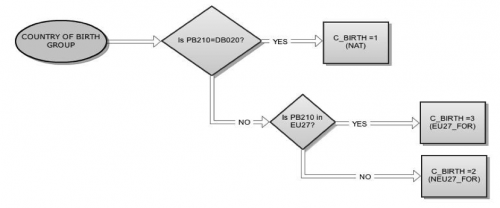
The respondent’s country of birth is recorded in the basic SILC variable PB210; this variable helps for the calculation of the country of birth group variable (C_BIRTH). The following country of birth groups are considered

• NAT (Declaring country), C_BIRTH=1
• FOR (Foreign countries), C_BIRTH=2-7
• NEU27_FOR (Foreign, non EU27-countries nor declaring country), C_BIRTH=2
• EU27_FOR (EU27-countries except declaring country), C_BIRTH=3
• NEU28_FOR (Non EU28-countries nor declaring country), C_BIRTH=4
• EU27_2019_FOR (EU28-countries except UK and declaring country), C_BIRTH=6
• NEU27_2019_FOR (Non EU27_2019-countries nor declaring country), C_BIRTH=4,7

The above country of birth groups using the basic variable PB210 are defined as follows:

From 2009 onwards, the following country of birth groups are also considered:

• EU28_FOR (EU28-countries except reporting country)
• NEU28_FOR (Non EU28-countries nor reporting country)

From 2019 onwards, the following country of birth groups are also considered:

• EU27_2019_FOR (EU27_2019-countries except reporting country)
• NEU27_2019_FOR (Non EU27_2019-countries nor reporting country)

→ SAS program: VAR_C_BIRTH_CIP_SHIP.sas

Country of birth of parents

The country of birth of parents (C_ΒΙRTH) uses the following basic SILC variables: FC_ΒΙRTH (father’s country of birth), MC_BIRTH (mother’s country of birth), RB220 (ID of the father) and RB230 (ID of the mother).

The following country of birth groups are considered

• NAT (Reporting country), C_ΒΙRTH =1
• FOR (Foreign country), C_ΒΙRTH =2
• OTH (Other), C_ΒΙRTH =-1

The country of birth of parents calculation is described below.

• if (FC_ΒΙRTH =1 and MC_BIRTH = 1) or (FCIT_SHIP =1 and MC_BIRTH is missing and RB230_F is not applicable) or (FCIT_SHIP is missing and RB220_F is not applicable) then C_ΒΙRTH = 1
• if FCIT_SHIP >1 or MC_BIRTH >1 then C_ΒΙRTH = 2
• else C_ΒΙRTH = -1

Employment security transition level (W_SEC)

The employment security transition level variable is concerned with the definition of ‘good’ and bad employment security transitions. Currently ‘good’ transitions increasing the employment security compared to last year are the following:

Last year working status	Current year working status	W_SEC (Value)
Employees with a permanent contract	Employees with a permanent contract	100
Employees with a temporary contract	Emploees with a permanent or temporary contract or self – employed	200
Emploees self – employed	Emploees with a permanent or temporary contract or self – employed	300
Unemployed persons	Emploees with a permanent or temporary contract or self – employed or students	400
Student	Emploees with a permanent or temporary contract or self – employed or students	500
Retired		600
Other inactive persons	Employees with a permanent or temporary contract or self – employed or students or unemployed or other inactive persons	700

Any labour market transition not included in the above table is considered a bad employment security transition decreasing the employment security compared to last year. For bad employment security transition the variable W_SEC takes the value -1000. The security transitions presented in the above table make use of the derived variable Adjusted self – defined current economic status (PL31).

→ SAS program: L_lvhl33.sas

Highest Education Level of Children's Parents (HHISCED)

Highest educational level of children’s parents refers to children living in a household with one or both parents and to the highest level of education attained by (at least one of) the parents. Data are classified according to the International Standard Classification of Education (ISCED): low education corresponds to ISCED levels 0-2 (pre-primary, primary and lower secondary education); medium education corresponds to ISCED levels 3 and 4 (upper secondary and post-secondary non-tertiary education) and high education corresponds to ISCED levels 5 and 6 (tertiary education).

The algorithm for highest educational level of children’s parents uses the following basic SILC variables: FPE040 (highest ISCED level attained by the father) and MPE040 (highest ISCED level attained by the mother).

if [math]FPE040\geq\;MPE040[/math] then [math]HHISCED=\;FPE040[/math]

if [math]MPE040\geq\;FPE040[/math] then [math] HHISCED =\;MPE040[/math]

Otherwise the Educational level of children’s parents is missing.

The calculation of the HHISCED variable based on the data coming from the EU-SILC 2011 ad hoc module on ‘Intergenerational transmission of disadvantages’ is the same. However, the variables PT110 and PT120 of the 2011 ad hoc module are used, denoting the the highest ISCED level attained by the father and the highest ISCED level attained by the mother respectively.

→ SAS program: VAR_HHISCED.sas

Longitudinal weight estimate - four year duration (RB064)

The variable RB064e is an estimation of the longitudinal weight RB064 for countries for which the real longitudinal weigh (RB064) is missing. The calculation algorithm for the fictive longitudinal weight (RB064e) uses the following auxiliary variables:

• RB060s - The sum of the personal base weight RB060 (constructed)
• RB063s - The sum of the longitudinal weight RB063 (constructed)
• RB064s - The sum of the longitudinal weight RB064 (constructed)

The calculation of variables RB060s, RB063s and RB064s is described below.

[math]RB060_s=\sum \limits_{i}RB060_i[/math]

[math]RB063_s=\sum \limits_{i}RB063_i[/math]

[math]RB064_s=\sum \limits_{i}RB064_i[/math]

The estimation for the longitudinal weight RB064e is calculated as:

[math]RB064_e=\left\{\begin{matrix} RB063\times\;(\frac{RB060_s}{RB063_s}),\;if\;RB064_s=0 \\ RB064,\;if\;RB064_s\neq 0 \end{matrix}\right.[/math]

→ SAS program: VAR_ARPTXXip_RB064e.sas

Longitudinal weight estimate - two year duration (SEL_WGT)

The variable SEL_WGT is an estimation of an equivalent to the longitudinal weight RB062 for selected respondents. The algorithm calculating the weight (SEL_WGT) uses the following relevant basic SILC variables: RB062 (longitudinal weight – two year duration), PB080 (personal base weight for selected respondent) as well as the following auxiliary variables:

• SUM_RB062 - The sum of the longitudinal weight RB062 (constructed)
• SUM_PB080 - The sum of the personal base weight for selected respondent PB080 (constructed)

The calculation of variables SUM_RB062, SUM_PB080 is described below.

[math]SUM\_RB062=\sum\limits_{i}RB062_i[/math]

[math]SUM\_PB080=\sum\limits_{i}PB080_i[/math]

Following the above definitions the estimation for the longitudinal weight RB062 is calculated as:

[math]SEL\_WGT=\left\{\begin{matrix} 0,\;if\;PB080=0\;or\;RB062=0 \\ PB080\times\;(\frac{SUM\_RB062}{SUM\_PB080}),\;if\;RB062\gt 0\;and\;PB080\gt 0 \\ RB062,\;if\;PB080=RB062\neq 0\;and\;(RB062\lt 0\;or\;PB080\lt 0) \end{matrix}\right.[/math]

It should be noted that SEL_WGT (from 2014) refers to all current household members aged 16 over (for countries using selected respondent design).

→ SAS program: VAR_SEL_WGT.sas

Qualification transition level (W_QUAL)

The qualification transition level variable is concerned with the definition of ‘good’ and bad labour market transitions. Currently ‘good’ transitions are the ones from unemployment/inactivity to employment or movements from low paid to high paid jobs. Qualification transition level variable takes values -1 and 1 for bad and good transitions respectively whereas for the rest of transitions take a zero value. The qualification transitions we consider as well as their characterisation based to the value of W_QUAL variable are presented in the following table:

Last year working status	Current year working status	Change in employment income decile	W_QUAL (Value)
Employed	Employed	Better income decile	1
Employed	Student	-	1
Unemployed	Employed or student	-	1
Student	Employed or student	-	1
Other inactive persons	Employed, student or unemployed	-	1
Employed	Employed	Same income decile	0
Unemployed	Unemployed	-	0
Othet inactive persons	Othet inactive persons	-	0
Employed	Employed	Worse income decile	-1
Employed	Unemployed	-	-1
Unemployed	Other inactive persons	-	-1
Student	Other inactive persons	-	-1

→ SAS program: L_lvhl35.sas

Weight for the Respondents (RES_WGT)

The variable RES_WGT is a weight assigned to each selected respondent. The algorithm for the calculation of the weight (RES_WGT) uses the following relevant basic SILC variables: PB040 (Personal cross-sectional weight) and PB060 (Personal cross-sectional weight for selected respondent).

RES_WGT is calculated as follows:

If PB060 >0 then RES_WGT=PB060

else RES_WGT=PB040

It should be noted that both PB040 and PB060 refer to all current household members aged 16 and over.

→ SAS program: VAR_RES_WGT.sas

Worked months

The calculation of the total months worked for the working age members of the household is presented schematically below:

The above calculation makes use of the derived variables Activity Status (ACTSTA) and Age.

→ SAS program: IW06.sas

Linking variables

Linking variables are identification variables of the whole survey.

• Year of the survey (depending on the file that is transmitted to Eurostat: DB010, HB010, PB010, RB010)
• Country (depending on the file that is transmitted to Eurostat: DB020, HB020, PB020, RB020)
• Household ID (depending on the file that is transmitted to Eurostat: DB030, HB030, PB030, RB030)

More information on these variables is provided in the Methodological guidelines and description of EU-SILC target variables.

Auxiliary variables

Auxiliary variables are computed variables that refer to the whole statistical population, rather than to distinct statistical units-observations. These variables result from Eurostat's calculations (based on the SAS scripts developed) and include statistical measures, thresholds, etc.

These variables are listed below, along with the description for their computation.

Gini coefficient

Let EQ_INCi be the equivalised disposable income of person i and Weight’i the weight for person i

Persons have to be sorted according to EQ_INC (sorting order: lowest to highest value), then by household identification number and personal identification number in order to obtain a unique ordering.

As each individual weight' i of person i in the sample represents the number of persons in the population with identical (income) characteristics, our method needs to be neutral to be the number of actual sample observations with a particular income, i.e. the slope of each of the linear functions the Lorenz curve is composed of should be indifferent to the amount of observations on each of these linear functions.

Thus, although we need to order incomes in increasing order and not multiply by weights, because no matter what type of aggregation we deal with and what proportions of the population are represented with each observation, should not affect the fact that the Lorenz curve should non-decreasing in slope with increasing proportion of the population represented by weight'i.

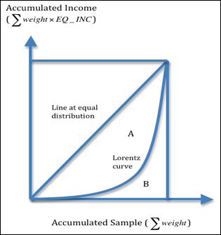
So, on the y-axis, we need to multiply for each observation the corresponding income observation with its weight, so that on the y-axis we do not have accumulated sample income but [math]\sum \limits_{i=1}^{n}EQ\_INC_i\times\;weight'_i[/math]. On the y-axis, proportions of income of the population should be represented. This is given by [math]\sum \limits_{j=1}^{n}EQ\_INC_j\times\;weight'_j[/math] and not by [math]\sum \limits_{j=1}^{n}EQ\_INC_j[/math]. On the x-axis coordinates are represented by [math]\sum\limits_{j=1}^{n}weight'_j[/math].

The area A+B (triangle below the line of equal distribution) will be given by:

[math]A+B=\frac{\sum\limits_{i=1}^{n}(EQ\_INC_i\times\;weight'_i)\times\sum\limits_{i=1}^{n}weight'_i}{2}[/math]

and the area under the Lorenz curve B will be given by:

[math]B=\sum\limits_{i=1}^{n}[(\sum\limits_{j=1}^{i}EQ\_INC_i \times\;weight'_i -0.5\times\;EQ\_INC_i times\;weight'_i )\times\;weight'_i ][/math]

The Gini coefficient is calculated as:

[math]G=\frac{A}{A+B}=1-\frac{B}{A+B}[/math]

Median equivalised disposable income level after social transfers (MEDIAN20)

Persons have to be sorted according to their Equivalised disposable Income (EQ_INC) (after social transfers) (sorting order: lowest to highest value, household identification number and personal identification number). The median is then calculated as:

[math]EQ\_INC20_{MEDIAN}=\left\{\begin{matrix} \frac{1}{2} (EQ\_INC20_j+EQ\_INC20_{j+1}),\;if\;\sum \limits_{i=1}^{j}RB050a_i=\frac{1}{2}\sum \limits_{i=1}^{n}RB050a_i\\ EQ\_INC20_{j+1},\;if\;\sum \limits_{i=1}^{j}RB050a_i\lt \frac{1}{2}\sum \limits_{i=1}^{n}RB050a_i\lt \frac{1}{2}\sum \limits_{i=1}^{j+1}RB050a_i \end{matrix}\right.[/math]

where

[math]EQ\_INC20_i[/math] = Equivalised disposable Income (EQ_INC) (after social transfers) of person i

[math]RB050a_i[/math] = is the Adjusted cross sectional weight (RB050a) for person i

[math]n[/math] = number of household members in the sample

Note: Households (and persons therein) with missing equivalised disposable income (EQ_INC20) are excluded. The median is calculated on the level of the individuals in the sample.

→ SAS program: VAR_ARPTXX.sas

Median working income (MEDIAN_INCWRK)

Persons have to be sorted according to their Working Income (INCWRK) (sorting order: lowest to highest value, household identification number and personal identification number). The median is then calculated as:

[math]INCWRK_{MEDIAN}=\left\{\begin{matrix} \frac{1}{2} (INCWRK_j+INCWRK_{j+1}),\;if\;\sum \limits_{i=1}^{j}PB040_i=\frac{1}{2}\sum \limits_{i=1}^{n}PB040_i\\ INCWRK_{j+1},\;if\;\sum \limits_{i=1}^{j}PB040_i\lt \frac{1}{2}\sum \limits_{i=1}^{n}PB040_i\lt \frac{1}{2}\sum \limits_{i=1}^{j+1}PB040_i \end{matrix}\right.[/math]

where

[math]INCWRK_i[/math] = Working income (INCWRK) of person i [math]n[/math] = number of persons (household members) [math]PB040_i[/math] = is the personal cross – sectional weight for person i

Median pension income (MEDIAN_INCPEN)

Persons have to be sorted according to their Pension Income (INCPEN) (sorting order: lowest to highest value, household identification number and personal identification number). The median is then calculated as:

[math]INCPEN_{MEDIAN}=\left\{\begin{matrix} \frac{1}{2} (INCPEN_j+INCPEN_{j+1}),\;if\;\sum \limits_{i=1}^{j}PB040_i=\frac{1}{2}\sum \limits_{i=1}^{n}PB040_i\\ INCPEN_{j+1},\;if\;\sum \limits_{i=1}^{j}PB040_i\lt \frac{1}{2}\sum \limits_{i=1}^{n}PB040_i\lt \frac{1}{2}\sum \limits_{i=1}^{j+1}PB040_i \end{matrix}\right.[/math]

where

[math]INCPEN_i[/math] = Pension income (INCPEN) of person i

[math]n[/math] = number of persons (household members)

[math]PB040_i[/math] = is the personal cross – sectional weight for person i

Mean equivalised disposable income level after social transfers

The mean of the Equivalised Disposable Income (EQ INC) (after social transfers) for the total number of household members in the sample is calculated as:

[math]EQ\_INC20 \left[MEAN \right]=\frac{\sum\limits_{i=1}^{n}EQ\_INC20_i\times\;RB050a_i }{\sum\limits_{i=1}^{n}RB050a_i }[/math]

where:

[math]EQ\_INC20_i[/math] = Equivalised disposable Income (EQ_INC) (after social transfers) of person i

[math]RB050a_i[/math] = is the Adjusted cross sectional weight (RB050a) for person i

[math]n[/math] = number of household members in the sample

Note: Households (and persons therein) with missing equivalised disposable income (EQ_INC20) are excluded. The mean is calculated on the level of the individuals in the sample.

Risk of poverty threshold (ARPTXX)

The at-risk-of-poverty threshold is calculated as the XX percentage of the median or mean value of the Equivalised disposable Income (EQ_INC) after social transfers (EQ_INC20).

[math]ARPTXX=XX\%\times\;EQ\_INC20_{MEDIAN}[/math]

[math]ARPTMXX=XX\%\times\;EQ\_INC20_{MEAN}[/math]

The usual definition defines at-risk-of-poverty threshold as 60% of the equivalised median income after social transfers so the value ARPT60 threshold is the most commonly used. Different thresholds (ARPT40, ARPT50, ARPT70, ARPTM40, ARPT50, ARPT60) are also calculated to derive different poverty rates.

→ SAS program: VAR_ARPTXX.sas

Direct access to

Other articles

Tables

Database

Dedicated section

Publications

Methodology

Legislation

Visualisations

External links

Other articles

• EU statistics on income and living conditions (EU-SILC) methodology (overview of all articles)

Main tables

• Income and living conditions (t_ilc)

Database

• Living conditions and welfare (livcon), see:

Income and living conditions (ilc)

People at risk of poverty or social exclusion (Europe 2020 strategy) (ilc_pe)

Main indicator - Europe 2020 target on poverty and social exclusion (ilc_peps)

Dedicated section

Income and living conditions (ilc)

Publications

• The continuity of indicators during the transition between ECHP and EU-SILC
• Comparative EU quality reports
• Modules: assessment of implementation

Methodology

• Income and living conditions (ilc)] (ESMS metadata file — ilc_esms)
• Operation guidelines
• Methodological guidelines and description of EU-SILC target variables

Notes